Resistance temperature detectors : Basics

The principle of resistance temperature detectors (RTD) is based on the variation of electrical resistance of metals with temperature. For this purpose several metals are used, namely, platinum, copper, nickel. When temperature increases the resistance of these metals increases. Temperature function of resistance for metals in a narrow temperature interval can be expressed by a relationship:

(1)

where:

R_ϑ and R₀        - are the values of electrical resistance of a metal conductor at temperatures ϑ and 0,̊C, respectively, Ohm;

α                      - thermal coefficient of electrical resistance, 1/̊C .

For metals this coefficient is positive. Fig.1 shows relationship between resistance of platinum and copper RTD and temperature.

Platinum RTDs are used for temperature measurements from -220 to 850 ^oC (they are used as reference RTDs, as well), copper RTD - from -50 to 150 ^oC, and Nickel RTD - from -215 to 320 ^oC.

Figure 1: Resistance vs temperature for platinum and copper RTD.

Fig. 2 shows the assembly of RTDs. Sensitive elements of RTDs are made of a thin wire 1 with outside diameter equal to 0.025 mm (platinum RTD) and 0.1 mm (copper RTD) double wounded (non-inductive) on a micaceous or porcelain stem 2. For mechanical strength the sensitive element is placed in the ceramic insulator tube 3 filled by extremely fine granular powder; extension wires are placed in the ceramic insulator 4, and entire assembly is covered by a protective sheath of stainless steel 5. The space between the sheath and ceramic insulator is filled by ceramic packing powder 6. To avoid contact of sensitive element with environment, sensitive assembly is protected by high-temperature hermetic seal 7. The contact between the wire of the sensitive element and the ceramic encapsulation permits a rapid speed of response.

Figure 2: RTD assembly.

For measurements of resistance of RTDs several methods are used. Among them the most widely used is a method employing a Wheatstone bridge (Figure 3). In this case RTD is connected to the bridge by two connecting cables (conductors). The bridge is powered by direct current power supply in the points "a" and "b". RTD is immersed in the media, which temperature to be measured. When this bridge is in balance, then there is no voltage between points "c" and "d", and zero-indicator (ZI) shows no current. For this condition we can write the following equation:

(2)

or

(3)

where:

R₁ and R₂                    - electrical resistance of two invariable resistors, usually, R₁=R₂, Ohm;

R_ϑ                                - electrical resistance of RTD, Ohm;

R_c                                - electrical resistance of a connecting cable, Ohm;

R_sr                                - electrical resistance of a slide (variable) resistor, Ohm.

Figure 3.: Two-conductor connecting.   Figure 4: Three-conductor connecting.

As follows from these equations, the certain position of a slide of the variable resistor (ie, certain value of R_sr) corresponds to each value of a measuring temperature (ie, for each value of R_ϑ) at any balance condition of the bridge. Therefore, the scale of the bridge may be calibrated in degrees Celsius.

For a two-conductor connecting scheme (see Fig.3), variation of an ambient temperature will effect values of an electrical resistance of connecting cables R_cand, therefore, the results of measurements will be erroneous.

With all resistance temperature detectors a three-conductor connection scheme is recommended (see Fig. 4). One conductor is common to both sides of the bridge, while other two connect the RTD to each side of the bridge. Any change in the cable temperature (as the result of variations in ambient temperature) will be cancelled because the resistance of both sides of the bridge change by the same value (providing three connecting cables are at the same temperature).

A four-conductor connection scheme is used when very accurate measurements of temperature are required, up to ±0.01 °C of accuracy.

 Derivation of a balanced condition for a Wheatstone Bridge

Below I give you the derivation of the balanced condition for a Wheatstone bridge. Figure 4a shows a circuit of five electrical resistors connected to form the Wheatstone bridge.

Figure 4a.: Wheatstone bridge.

Here we use two Kirchoff’s Laws. The first Kirchoff’s law says: the total current flowing into any junction is equal to the total current flowing out of this junction. The second Kirchoff’s law states: the total change in potential around any closed circuit loop is equal to zero.

For the second Kirchoff’s law we should be sure to include the sign of potential energy correctly: the potential decreases around a resistor in the direction of current flow and increases in the direction opposite to current flow; potential increases from negative to positive terminals of the battery.

Below I give you two different methods for the derivation of the balanced condition for a Wheatstone bridge.

Now, let’s consider several closed circuit loops and apply the above law to them.

a. First method

1. Loop            e-a-b-c-f-e :

(4)

2. Loop            a-b-g-d-a :

(5)

3. Loop            b-c-d-g-b :

(6)

Here, U is a dc voltage, and U≠ 0.

So, we have three equations with 3 unknowns - I₁; I₃ and I₅.

(7)

(8)

                                                                                                                                                                                                           

(9)

Now we combine terms with I₁; I₃ and I₅.

(10)

(11)

(12)

Now we evaluate the determinant of the matrix developed using this set of equations:

(13)

In the case of the Wheatstone bridge the resistance R₅ is substituted by an ampmeter. Ampmeters have a negligibly small resistance, so we can write that R₅ = 0. With this condition we can re-write (13) as follows:

(14)

Because all R_i > 0 we have that ∆ > 0 and ∆ ≠ 0.

For current I₅ we have:

(15)

Now we can evaluate the value of the current, which flows through an ammeter as follows:

(16)

.                             

We know that a balanced condition is when current I₅ = 0, and because ∆ > 0, and ∆ ≠ 0 and U ≠ 0, we can give an expression for the balanced condition for the Wheatstone bridge as follows:

(17)

or, finally,

(18)

b. Second method

When the bridge is balanced, ie I₅ = 0, and current

1. Loop            e-a-b-c-f-e :

(19)

or,

(20)

2. Loop            e-a-d-c-f-e :

(21)

or,

(22)

Assume point f is at earth potential, then potential at point  e is equal to U_a = U. Potential at point b is equal to

(23)

Potential at point d is equal to

(24)

Potential difference between points b and d is equal to

(25)

Using equations (20) and (22) we can get:

                                                                                                                           (26)

and   

(27)

Substitute equations (26) and (27) into equation (25):

(28)

or,

(29)

or,

(30)

Since R₃ ≠ 0  and R₁ ≠ 0, then

(31)

We know for balanced condition I₅ = 0, then voltage U_bd = 0. Because U ≠ 0, then

(32)

or,

(33)

or,

(34)

So, finally, we get

(35)

Article Source:: Dr. Alexander Badalyan, University of South Australia

Read more...

Thermocouples : Basics

Seebeck in 1821 discovered that thermal electromotive force (t.e.m.f.) is generated in a closed circuit of two wires made of dissimilar metals if two junction are at different temperatures. One junction is inserted into a measuring media, and it is called a hot or measuring junction. Another one, called a cold or reference junction, is kept either at 0 °C or at ambient temperature and is connected to a measuring instrument (millivoltmeter). 

The electronic explanation of this phenomenon is as follows:

the density of conduction electrons in two dissimilar metals is different. So, in the case when metals are brought into contact (welded together), the free (or conduction) electrons will flow from the metal with high their density to the metal with low density of the conduction electrons. As the result of this drift, a potential difference is produced in the boundary between these two metals. This potential difference will stop the flow of electrons. Since the metals are different, so they will differently respond to temperature variations. In other words, the variation of temperature will change the density and velocities of free electrons in two metals differently. This will cause the change in the magnitude of the thermal electromotive force.

Figure 1: schematically shows a thermocouple and a measuring instrument.

Figure 1:      Thermocouple and measuring instrument.
1 - hot junction;              2 - metal A;                     3 - metal B;

4 - connection head;                 5 - extension wires;

6, 7 - positive and negative terminals, respectively, of a measuring instrument;

8 - measuring instrument.

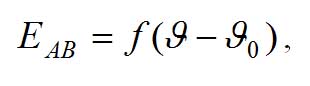
T.e.m.f. is proportional to the difference of temperatures between the two junctions. All tables, correlated t.e.m.f. of thermocouple (measured in mV) and temperature, are developed when the temperature of a cold junction is equal to 0 °C. T.e.m.f. is the function of temperature difference between the hot and the cold junctions:

                                       (1)

where:

E_AB               - t.e.m.f. developed by a thermocouple, mV;

ϑ and ϑ₀        - temperatures of the hot and the cold junctions of a thermocouple, ̊C.

If the temperature of the cold junction is kept constant (say at 0, ̊C), then t.e.m.f. is proportional to the temperature of the hot junction (the measuring temperature), ie

                                               (2)

In reality, in industrial environment, however, it is not possible (or is not convenient) to keep the temperature of the cold junction at 0, ̊C. Therefore, to evaluate the actual t.e.m.f. and, finally, the actual measuring temperature, we should introduce a correction. A final equation has the following form:

                                                         (3)

where:

E_AB(ϑ,ϑ₀)       - t.e.m.f. developed by a thermocouple when the temperature of the hot  junction is equal to ϑ  and the temperature of the cold junction is equal to ϑ₀ = 0, ̊C ,mV;

E_AB(ϑ_,ϑ'₀)        - t.e.m.f. developed by a thermocouple when the temperature of the hot junction is equal to ϑ and the temperature of the cold junction is equal to ϑ'₀ (different from 0, ̊C) – this t.e.m.f. is measured by a millivoltmeter, mV;

E_AB(ϑ_0,ϑ'₀)      - t.e.m.f. developed by a thermocouple when the temperature of the hot junction is equal to ϑ'₀ and the temperature of the cold junction is equal to ϑ₀ = 0_, ̊C ,mV.

There are various types of thermocouples:

• Platinum and Platinum - 10% Rhodium (type S) from -50 to 1765 °C;

• Platinum - 6% Rhodium and Platinum - 30% Rhodium (type B) from 0 to 1820 °C;

• Nickel - Chromium and Nickel - Aluminium (Chromel-Alumel, type K) from -270 to 1370 °C;

• Iron and Copper - Nickel (Iron - Constantan, type J) from -210 to 1200 °C;

• Copper and Copper - Nickel (Copper - Constantan, type T) from -270 to 400 °C;

• Nickel - Chromium and Copper - Nickel (Chromel - Constantan, type E) from -270 to 1000 °C.

Figure 2 presents experimental curves thermal electromotive force vs temperature for several types of thermocouples.

Figure 2: Experimental curves thermal electromotive force vs temperature.

Requirements imposed to the properties of metals used as electrodes for thermocouples are as follows:

• reproducibility of material, ie possibility of obtaining of metal wires with the same properties;

• resistance of metal electrodes should be small and have a weak relationship vs temperature;

• stability of a static characteristic E_AB = f(ϑ), ie recovery of properties after measurements;

• high sensitivity;

• correlation E_AB = f(ϑ) should be close to linear relationship as much as possible.

The highest sensitivity has thermocouple of Type J (Iron - Constantan): S= 0.055, mV/°C.

Article Source:: Dr. Alexander Badalyan, University of South Australia

Read more...

Piezoelectric Transducers

The conversion of electrical pulses to mechanical vibrations and the conversion of returned mechanical vibrations back into electrical energy is the basis for ultrasonic testing. The active element is the heart of the transducer as it converts the electrical energy to acoustic energy, and vice versa. The active element is basically a piece of polarized material (i.e. some parts of the molecule are positively charged, while other parts of the molecule are negatively charged) with electrodes attached to two of its opposite faces. When an electric field is applied across the material, the polarized molecules will align themselves with the electric field, resulting in induced dipoles within the molecular or crystal structure of the material. This alignment of molecules will cause the material to change dimensions. This phenomenon is known as electrostriction. In addition, a permanently-polarized material such as quartz (SiO2) or barium titanate (BaTiO3) will produce an electric field when the material changes dimensions as a result of an imposed mechanical force. This phenomenon is known as the piezoelectric effect.

The active element of most acoustic transducers used today is a piezoelectric ceramic, which can be cut in various ways to produce different wave modes. A large piezoelectric ceramic element can be seen in the image of a sectioned low frequency transducer. Preceding the advent of piezoelectric ceramics in the early 1950's, piezoelectric crystals made from quartz crystals and magnetostrictive materials were primarily used. The active element is still sometimes referred to as the crystal by old timers in the NDT field. When piezoelectric ceramics were introduced, they soon became the dominant material for transducers due to their good piezoelectric properties and their ease of manufacture into a variety of shapes and sizes. They also operate at low voltage and are usable up to about 300oC. The first piezoceramic in general use was barium titanate, and that was followed during the 1960's by lead zirconate titanate compositions, which are now the most commonly employed ceramic for making transducers. New materials such as piezo-polymers and composites are also being used in some applications.

The thickness of the active element is determined by the desired frequency of the transducer. A thin wafer element vibrates with a wavelength that is twice its thickness. Therefore, piezoelectric crystals are cut to a thickness that is 1/2 the desired radiated wavelength. The higher the frequency of the transducer, the thinner the active element. The primary reason that high frequency contact transducers are not produced is because the element is very thin and too fragile.

Characteristics of Piezoelectric Transducers

The transducer is a very important part of the ultrasonic instrumentation system. As discussed on the previous page, the transducer incorporates a piezoelectric element, which converts electrical signals into mechanical vibrations (transmit mode) and mechanical vibrations into electrical signals (receive mode). Many factors, including material, mechanical and electrical construction, and the external mechanical and electrical load conditions, influence the behavior of a transducer. Mechanical construction includes parameters such as the radiation surface area, mechanical damping, housing, connector type and other variables of physical construction. As of this writing, transducer manufacturers are hard pressed when constructing two transducers that have identical performance characteristics.

A cut away of a typical contact transducer is shown above. It was previously learned that the piezoelectric element is cut to 1/2 the desired wavelength. To get as much energy out of the transducer as possible, an impedance matching is placed between the active element and the face of the transducer. Optimal impedance matching is achieved by sizing the matching layer so that its thickness is 1/4 of the desired wavelength. This keeps waves that were reflected within the matching layer in phase when they exit the layer (as illustrated in the image to the right). For contact transducers, the matching layer is made from a material that has an acoustical impedance between the active element and steel. Immersion transducers have a matching layer with an acoustical impedance between the active element and water. Contact transducers also incorporate a wear plate to protect the matching layer and active element from scratching.

 

The backing material supporting the crystal has a great influence on the damping characteristics of a transducer. Using a backing material with an impedance similar to that of the active element will produce the most effective damping. Such a transducer will have a wider bandwidth resulting in higher sensitivity. As the mismatch in impedance between the active element and the backing material increases, material penetration increases but transducer sensitivity is reduced.

Transducer Efficiency, Bandwidth and Frequency

Some transducers are specially fabricated to be more efficient transmitters and others to be more efficient receivers. A transducer that performs well in one application will not always produce the desired results in a different application. For example, sensitivity to small defects is proportional to the product of the efficiency of the transducer as a transmitter and a receiver. Resolution, the ability to locate defects near the surface or in close proximity in the material, requires a highly damped transducer.

It is also important to understand the concept of bandwidth, or range of frequencies, associated with a transducer. The frequency noted on a transducer is the central or center frequency and depends primarily on the backing material. Highly damped transducers will respond to frequencies above and below the central frequency. The broad frequency range provides a transducer with high resolving power. Less damped transducers will exhibit a narrower frequency range and poorer resolving power, but greater penetration. The central frequency will also define the capabilities of a transducer. Lower frequencies (0.5MHz-2.25MHz) provide greater energy and penetration in a material, while high frequency crystals (15.0MHz-25.0MHz) provide reduced penetration but greater sensitivity to small discontinuities. High frequency transducers, when used with the proper instrumentation, can improve flaw resolution and thickness measurement capabilities dramatically. Broadband transducers with frequencies up to 150 MHz are commercially available.

Transducers are constructed to withstand some abuse, but they should be handled carefully. Misuse, such as dropping, can cause cracking of the wear plate, element, or the backing material. Damage to a transducer is often noted on the A-scan presentation as an enlargement of the initial pulse.


Article Source: www.ndt-ed.org

Read more...