Thermocouples : Basics

Seebeck in 1821 discovered that thermal electromotive force (t.e.m.f.) is generated in a closed circuit of two wires made of dissimilar metals if two junction are at different temperatures. One junction is inserted into a measuring media, and it is called a hot or measuring junction. Another one, called a cold or reference junction, is kept either at 0 °C or at ambient temperature and is connected to a measuring instrument (millivoltmeter). 

The electronic explanation of this phenomenon is as follows:

the density of conduction electrons in two dissimilar metals is different. So, in the case when metals are brought into contact (welded together), the free (or conduction) electrons will flow from the metal with high their density to the metal with low density of the conduction electrons. As the result of this drift, a potential difference is produced in the boundary between these two metals. This potential difference will stop the flow of electrons. Since the metals are different, so they will differently respond to temperature variations. In other words, the variation of temperature will change the density and velocities of free electrons in two metals differently. This will cause the change in the magnitude of the thermal electromotive force.

Figure 1: schematically shows a thermocouple and a measuring instrument.

Figure 1:      Thermocouple and measuring instrument.
1 - hot junction;              2 - metal A;                     3 - metal B;

4 - connection head;                 5 - extension wires;

6, 7 - positive and negative terminals, respectively, of a measuring instrument;

8 - measuring instrument.

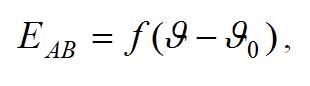
T.e.m.f. is proportional to the difference of temperatures between the two junctions. All tables, correlated t.e.m.f. of thermocouple (measured in mV) and temperature, are developed when the temperature of a cold junction is equal to 0 °C. T.e.m.f. is the function of temperature difference between the hot and the cold junctions:

                                       (1)

where:

E_AB               - t.e.m.f. developed by a thermocouple, mV;

ϑ and ϑ₀        - temperatures of the hot and the cold junctions of a thermocouple, ̊C.

If the temperature of the cold junction is kept constant (say at 0, ̊C), then t.e.m.f. is proportional to the temperature of the hot junction (the measuring temperature), ie

                                               (2)

In reality, in industrial environment, however, it is not possible (or is not convenient) to keep the temperature of the cold junction at 0, ̊C. Therefore, to evaluate the actual t.e.m.f. and, finally, the actual measuring temperature, we should introduce a correction. A final equation has the following form:

                                                         (3)

where:

E_AB(ϑ,ϑ₀)       - t.e.m.f. developed by a thermocouple when the temperature of the hot  junction is equal to ϑ  and the temperature of the cold junction is equal to ϑ₀ = 0, ̊C ,mV;

E_AB(ϑ_,ϑ'₀)        - t.e.m.f. developed by a thermocouple when the temperature of the hot junction is equal to ϑ and the temperature of the cold junction is equal to ϑ'₀ (different from 0, ̊C) – this t.e.m.f. is measured by a millivoltmeter, mV;

E_AB(ϑ_0,ϑ'₀)      - t.e.m.f. developed by a thermocouple when the temperature of the hot junction is equal to ϑ'₀ and the temperature of the cold junction is equal to ϑ₀ = 0_, ̊C ,mV.

There are various types of thermocouples:

• Platinum and Platinum - 10% Rhodium (type S) from -50 to 1765 °C;

• Platinum - 6% Rhodium and Platinum - 30% Rhodium (type B) from 0 to 1820 °C;

• Nickel - Chromium and Nickel - Aluminium (Chromel-Alumel, type K) from -270 to 1370 °C;

• Iron and Copper - Nickel (Iron - Constantan, type J) from -210 to 1200 °C;

• Copper and Copper - Nickel (Copper - Constantan, type T) from -270 to 400 °C;

• Nickel - Chromium and Copper - Nickel (Chromel - Constantan, type E) from -270 to 1000 °C.

Figure 2 presents experimental curves thermal electromotive force vs temperature for several types of thermocouples.

Figure 2: Experimental curves thermal electromotive force vs temperature.

Requirements imposed to the properties of metals used as electrodes for thermocouples are as follows:

• reproducibility of material, ie possibility of obtaining of metal wires with the same properties;

• resistance of metal electrodes should be small and have a weak relationship vs temperature;

• stability of a static characteristic E_AB = f(ϑ), ie recovery of properties after measurements;

• high sensitivity;

• correlation E_AB = f(ϑ) should be close to linear relationship as much as possible.

The highest sensitivity has thermocouple of Type J (Iron - Constantan): S= 0.055, mV/°C.

Article Source:: Dr. Alexander Badalyan, University of South Australia

Read more...

Filled thermal systems

Another class of thermometers that utilise the principle of expansion of substances with temperature is called filled thermal systems. Depending on the phase of the substance, which fills these devices, these systems are sub-categorised into gas-, liquid- and vapour-filled systems.

Gas-filled systems are based on a basic law of gases. If a gas is kept in a metallic bulb (or a container) at a constant volume, then if the temperature varies, so does the pressure according to the relationship

                                                                                              (1)

where:

P₁and T₁          - absolute pressure (Pa) and temperature (K) at state 1;

P₂and T₂          - absolute pressure (Pa) and temperature (K) at state 2;

β                   - thermal coefficient of pressure, equal to the volumetric thermal expansion coefficient, K^-1

Figure 1: Gas- or liquid-filled thermometer.       

Figure 1 schematically shows the design of a gas-filled thermometer. Gas (nitrogen or helium) 1 fills the thermal bulb 2, capillary tube 3 and Bourdon tube of a manometer 4. The thermal bulb (usually made of a stainless steel) is immersed in the measuring media. Variation of its temperature causes change in pressure of the gas in the system. The manometer measures this variation of pressure. The scale of the manometer is graduated in °C, but not in Pa. The length of the capillary tube (usually made of a stainless steel) varies from 0.6 to 60 m. The accuracy of measurements for these thermometers is greatly influenced by variation of ambient temperature (since it can change the pressure of a gas in the system). Two methods are used to reduce this effect:

• a thermal bimetallic temperature compensator is used in the manometer;

• an internal volume of the thermal bulb should be greater than that of the capillary tube, the ratio V_b/V_c (where V_b and V_c are volumes of the thermal bulb and of the capillary, respectively) may vary from 40 to 60; this can be achieved by reducing the internal diameter of the capillary tube or increasing the internal volume of the thermal bulb. The longer the capillary tube, the bigger the thermal bulb should be.

Therefore, gas-filled thermometers are not widely used in practice.

Depending on the measured temperature range, the system may be filled with a gas under pressure higher than atmospheric. That is why variations in atmospheric pressure have no effect on the indications of gas-filled thermometers.

Gas-filled thermometers have several advantages:

• they have the widest temperature range of all filled systems;

• as follows from the equation (1) these thermometers have uniform scales;

• they have the longest capillary length compared with other filled systems.

These thermometers are usually used for temperature measurement in the range from

-200 to 600 °C.

Figure 2: Vapour-pressure system.

Liquid-filled systems have similar design with gas-filled thermometers (see Fig. 1). Organosilicone liquids, propanol and mercury are used as thermometric liquids, which fill the entire system. Since the total volume of the thermal system is constant, then variation of temperature of the media, where the thermal bulb is immersed, causes variation in the pressure of the thermometric liquid. This variation in pressure is proportional to the variation of temperature. Therefore, scales of liquid-filled thermometers are uniform.

Several factors influence the accuracy during temperature measurements, namely:

• variation in ambient temperature;

• variation in pressure head;

• variation in atmospheric pressure.

In order to compensate the influence of variation of an ambient temperature it is necessary to increase the ratio internal volume of the thermal bulb/internal volume of the capillary tube, and employ thermal bimetallic compensators (see gas-filled thermometers). The error due to variation of an ambient temperature is bigger in the case of liquid-filled systems, compared to gas-filled systems. Therefore, the capillary length for liquid-filled systems can not exceed 10 m.

When the thermal bulb is placed below or above the manometer, results of such temperature measurements will not be correct. This is because of different pressure head of the liquid column compared with the case when this thermometer was calibrated (the manometer and the thermal bulb were placed on the same level). In this case the error can be eliminated by zero correction of manometer. The ultimate elevation distance between the thermal bulb and the manometer are given in the calibration certificate supplied with the liquid-filled thermometer.

To reduce influence of variation of atmospheric pressure, the system is filled with liquid under pressure from 0.5 to 2.0 MPa.

Here are the advantages of liquid-filled thermometers:

• small time lag;

• small dimensions of thermal bulb.

These thermometers are used for temperature measurement in the range from -150 to 300 °C.

Vapour/pressure systems (see Fig. 2) are filled by 2/3 of the volume of the thermal bulb 1 by liquid 2 which has a low boiling temperature, for example, freon (refrigerant), propylene, acetone, ethylbenzene, methyl chloride, etc. Another (upper) part of the thermal bulb and the capillary tube 3 is occupied by saturated vapour 4 of this liquid. Vapour pressure depends only on the temperature of saturated liquid in the thermal bulb, and therefore, does not depend on the variation of the ambient temperature (this is an advantage). Relationship between saturation pressure and temperature for liquids is non-linear (see Fig. 3). Hence, the scales of these thermometers are non-uniform, with more widely spaced increments at high temperatures. The length of the capillary tube usually does not exceed 25 m.

Disadvantages of vapour-pressure thermometers are as follows:

• narrow temperature range, from -50 to 300 °C;

• slow response time (time lag) of about 20 seconds;

• non-uniformity of the temperature scale.

Figure 3:. Saturation (vapour pressure) curve for methyl chloride.

Article Source:: Dr. Alexander Badalyan, University of South Australia

Read more...

Dynamic characteristic of liquid-in-glass thermometer (thermal capacitance of glass wall is included)

Its a derivation  part which is a continuation of the previous two post. Here the dynamic characteristics of liquid-in-glass thermometer by considering the thermal capacitance of glass wall is discussed.

Its better you read the previous two post before going through this, for better understanding:

• Liquid-in-glass thermometer : Introduction
• Dynamic characteristic of liquid-in-glass thermometer (thermal capacitance of glass wall not included)

Dynamic characteristic of liquid-in-glass thermometer (thermal capacitance of glass wall is included)

The heat energy balance:

(20)

Thermal capacitance of the glass walls is included.

a). The heat energy balance for mercury in the bulb:

Figure 1:. Liquid-in-glass thermometer.

(25)(26)(27)

We get the first order differential equation:

(28)

b). The heat energy balance for the glass wall has both inflow and outflow of heat:

(29)(30)

(31)(32)

(33)

Let ∆t→0, then

(34)

Substitute (28) into (34) and after manipulations we get:

(35)

or

(36)

Equation (36) is a second-order differential equation.

C_g                - thermal capacitance of glass bulb, J/K;

c^g_p               - specific heat of glass, J/(kg*K);

M_g                - mass of glass bulb, kg;

∆Q^g_accum        - amount of heat energy accumulated by glass bulb during a period of time ∆t,J;

∆Q^g_in            - amount of heat energy transferred to glass bulb from fluid during a period of time ∆t, J;

∆Q^g_out           - outflow of heat energy from glass bulb during a period of time ∆t, J;

R_f,g               - thermal resistance of fluid film and glass wall, K/W;

R_g,m              - thermal resistance of glass and mercury film, K/W;

T_g                - temperature of glass, K.

(37)

(38)

where,

A_g                - heat transfer surface area, m²;

h_f,h_m            - film coefficients of fluid and mercury, respectively, W/(m²*K);

k_g                 - thermal conductivity of glass, W/(m*K);

x_g                 - thickness of glass wall, m.

Transfer function is as follows:

(39)

where,                   τ_1,2 = R_fl,gC_m..

Let,    τ₁ τ₂ =τ²,       (39)          and    τ₁₊ τ₂₊ τ_1,2= 2 ζτ.   (40)

Then, 

(41)

Let:    T'_fl = A - step change, and ζ = 1. Then we have:

(42)

Use inverse Laplace transform:

(43)

Let:    A= 10^oC and τ = 85,s. Then we can plot a transient response of this thermometer to a step change in the input variable (see Figure 2).

Figure 2:. Transient response of liquid-in-glass thermometer.

Article Source:: Dr. Alexander Badalyan, University of South Australia

Read more...

Dynamic characteristic of liquid-in-glass thermometer (thermal capacitance of glass wall is not included)

This post describes the dynamic characteristics of liquid-in-glass thermometer which contains a derivation part using the heat energy balance equation.Its the continuation of the previous post titled 'Liquid-in-glass Thermometer'. 

Dynamic characteristic of liquid-in-glass thermometer (thermal capacitance of glass wall is not included):

The heat energy balance for mercury in the bulb:

(1)

Thermal capacitance of the glass walls is neglected.

(8)(6)(7)

Let Dt®0, then we can get a first order differential equation:

(9)

Explanations of variables used in the above equations is given below:

C_m                - thermal capacitance of mercury, J/K;

C_p^m              - specific heat of mercury, J/(kg*K);

M_m               - mass of mercury, kg;

∆Q^m_accum.       - amount of heat energy accumulated by mercury during a period of time ∆t, J;

∆Q^m_in            - amount of heat energy transferred to mercury during a period of time ∆t, J;

∆Q^m_out           - outflow of heat energy from mercury during a period of time ∆t, J;

R_f,m              - thermal resistance between mercury and outside fluid,K/W;

∆t                 - period of time, s;

T_m                - temperature of mercury, K;

∆T_m/∆t         - rate of change of temperature of mercury, K/s;

dT_m/dt         - instantaneous rate of change of temperature of mercury, K/s;

T_fl                - temperature of the fluid outside the bulb, K.

(10)

A_g                - heat transfer surface area, m²;

h_fl,h_m            - film coefficients of fluid and mercury, respectively, W/(m²*K);

k_g                 - thermal conductivity of glass, W/(m*K);

x_g                 - thickness of glass wall, m.

Differential equation with variables in deviation form:

(11)(12)

Let:    T'_fl = A - step change. Then we have:

(13)(14)

(15)

Use inverse Laplace transform:

(16)

where,

τ = R_f,mC_m      - time constant, s.  Let:   A=10°C;       

          R_f,m = 131, K/W;               C_m = 0.56, J/K.

Figure 2 shows a dynamic response of this thermometer to a step change in temperature.

Figure 2.: Dynamic response of liquid-in-glass thermometer to a step change in temperature.

From equation (12) we can get:

(17)(18)

Using a block diagram in Figure 3 we can get the following expression for a transfer function:

Figure 3.: Block diagram of a thermometer.

(19)

Article Source:: Dr. Alexander Badalyan, University of South Australia

Read more...

Liquid-in-glass thermometers

These thermometers are used for temperature measurements from -200 to 750 °C. They are contact-type thermometers. Fig. 1 shows the principle of their design.

Figure 1.:  Liquid-in-glass thermometer

This thermometer consists of a glass bulb 1, which is connected with a glass capillary tube 2. A scale 3 in degrees of Celsius or Fahrenheit is placed behind the capillary tube. The bulb, the capillary tube and the scale are placed in a glass tube 4 to protect them against the damage. A thermometric liquid 5 fills the bulb and a part of the capillary tube. The operational principle of these thermometers is based on the difference between the volume expansion of liquids and glass with temperature. The relationship that governs the operation of this device is

where,        

V_T                - volume of liquid at temperature T_, m³;

V_T                - volume of liquid at temperature T₀, m³;

∆T= T-T₀       - difference of temperatures, K;

ᵦ               - volumetric thermal expansion coefficient, 1/K.

The volumetric thermal expansion coefficient of glass is much less than that of liquids. The variation of temperature (up and down) of the bulb causes liquid in the system to expand or decrease its volume, respectively. As a result of such changes (the internal volume of the glass bulb and the glass capillary varies negligible), the length of the liquid column in the capillary tube goes up or down proportionally to the variation of temperature.

The type of thermometric liquid depends on the lower and upper limits of the measuring temperature range. Table  presents the most common types of liquids used in these types of thermometer.

Table : Types of thermometric liquids.

Liquid	Temperature range, °C
	From	To
Mercury	-35	750
Toluene	-90	200
Ethanol	-80	70
Kerosene	-60	300
Petroleum Ether	-120	25
Pentane	-200	20

Among these liquids mercury is the most widely used, because:

• mercury is easy obtainable with high chemical purity;

• mercury does not wet glass (this increases the accuracy of measurement/ reading);

• mercury remains in liquid state in a wide temperature range.

Among disadvantages inherent to mercury-in-glass thermometers we can mention the following:

• mercury is a poisonous element, which affects the central and peripheral nervous system, its vapour is the most toxic;

• small volumetric thermal expansion coefficient for mercury, therefore, mercury is used in thermometers with capillaries of small internal diameter;

The solidifying point of mercury, ie 38 °C, limits the lowest temperature that can be measured by mercury-in-glass thermometers. The upper temperature is determined by the temperature at which glass still retains its solid properties. This temperature is equal about 600 °C for glass, and about 750 °C for silicon glass.

When air above mercury in the capillary is removed, a mercury-in-glass thermometer can be used at temperatures below 300 °C, because the boiling temperature of mercury at atmospheric pressure is equal 356.9 °C. In order to increase this temperature range it is necessary to increase the boiling temperature of mercury (saturation temperature). This can be achieved by increasing pressure in the capillary. Usually, the space above mercury in the capillary is filled by inert gas (such as nitrogen, argon) under pressure.

Liquid-in-glass thermometers with organic thermometric liquids are used for temperature measurements from -200 to 200 °C.


 One advantage of these thermometers is:

• a higher volume thermal expansion coefficient comparing with that for mercury (six times higher in average).

Disadvantage of thermometers with organic liquids is:

• these liquids wet glass, therefore, in order to increase the accuracy of measurement/reading, glass capillaries with bigger internal diameters (up to 1 mm) are used.

Advantages of liquid-in-glass thermometers are as follows:

• they are simple in design;

• they are relatively highly accurate in temperature measurement.

There are several disadvantages inherent to liquid-in-glass thermometers

• they are fragile;

• it is difficult to perform readings due to low visibility of the scale;

• they are not capable of distance transmission of a measuring signal, therefore, they are used as locally placed devices;

• impossibility to repair;

• high values of time lag;

• low visibility of mercury in the capillary.


Article Source:: Dr. Alexander Badalyan, University of South Australia

Read more...